Introduction

Introduction

Concept of PyTorchDecomp

In data science, we sometimes deal with thousands to millions of high-dimensional data (e.g., images, omics). Usually when machine learning is performed on such high-dimensional data, the data is projected once to a lower dimension to reduce the effects of the curse of dimensionality, and then applied for downstream learning (further dimensionality reduction, data reconstruction, clustering, predictive model building, optimal transport, etc.).

This dimensionality reduction step is often performed independently of downstream learning as a pre-processing step (Figure 1). However, in such cases, the unsupervised dimensionality reduction is performed without being aware of subsequent learning, which may lead to the extraction of patterns from the data that are not needed for subsequent learning. In the deep machine learning field, “End-to-End” modeling is used to unify such pre-processing and downstream learning as a single model. PyTorchDecomp follows this deep machine learning technique by combining dimensionality reduction and subsequent learning based on the PyTorch framework in a End-to-End manner (Figure 1).

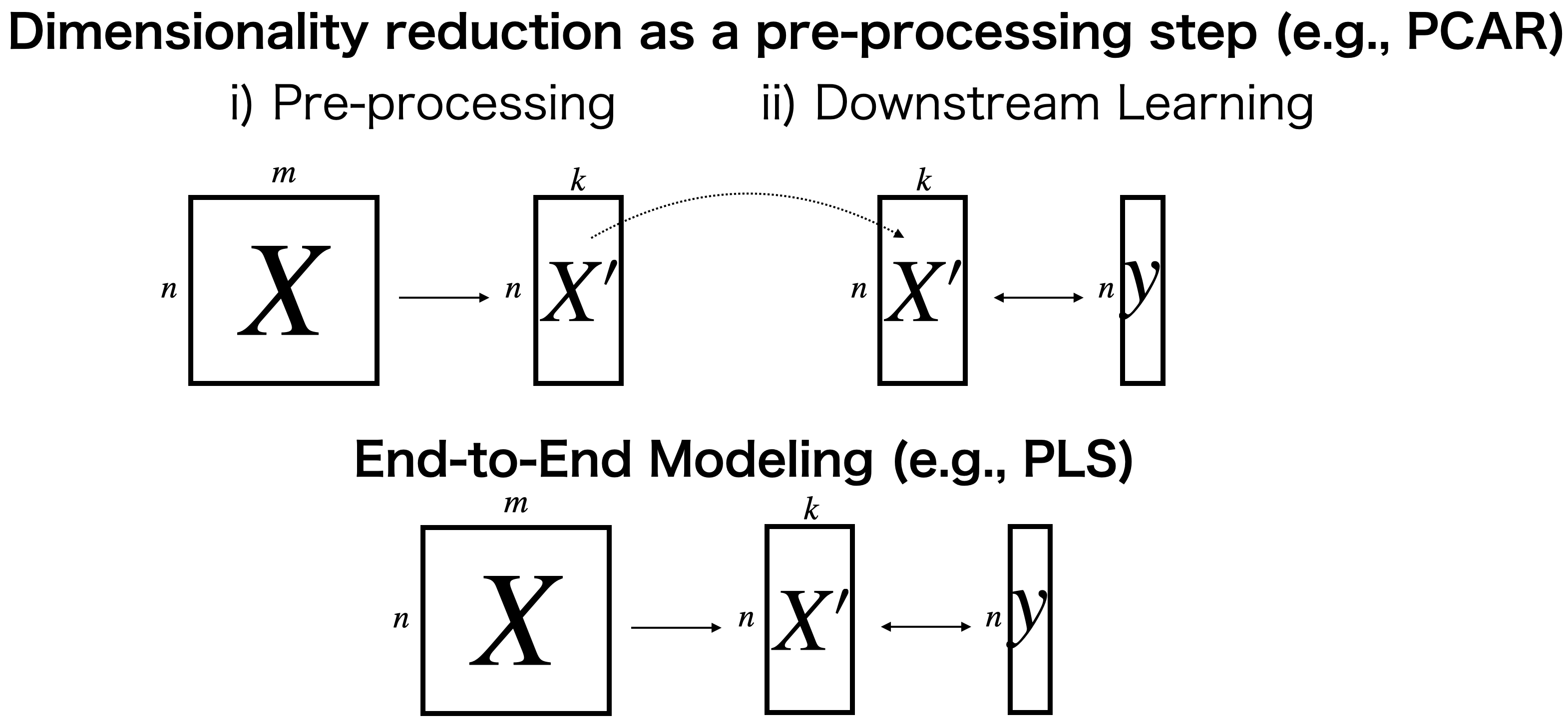
With PyTorchDecomp, an unsupervised dimensionality reduction model can be immediately converted to the supervised version. For example, consider PCA regression (PCAR), in which high-dimensional data are subjected to dimensionality reduction by PCA, followed by linear regression. In PCA as the pre-processing step, the loading matrix to project the data from a higher dimension to a lower dimension is learned to maximize the variance of the scores in the lower dimension, but maximizing variance does not always contribute to better predictive performance in subsequent regression because of outlier samples and subpopulations that do not follow labels. On the other hand, PyTorchDecomp can be used to treat dimensionality reduction and subsequent regression in an End-to-End manner. For example, in PyTorchDecomp, PCAR can be easily converted to Partial Least Squares (PLS), which can use both high-dimensional data and the corresponding label data to learn a projection matrix such that the covariance between them is maximized (!!! Link to Tutorial 3!!!) .

Why Matrix Decomposition in PyTorch?

Since the research communities of matrix factorization and deep learning are considered to be different, it is possible to import discussions between different research communities to each other, which could have the following advantages.

The advantages of using PyTorchDecomp from the point of view of users of matrix factorization algorithms may include the following:

• Easy to speed up: Parameter optimization in PyTorch is based on iterational computations, such as the (stochastic) gradient method. This is often faster than conventional parameter optimization based on matrix diagonalization or inverse matrix computation that has been used in multivariate analysis field, and is easier to apply to large data sets. In addition, PyTorch supports GPU computation, which is expected to further speed up the process.

• Easy to extend the model: PyTorch optimizes parameters based on automatic differentiation. This differs from the conventional multivariate analysis approach, in which the parameter’s derivative of the objective function (gradient) is obtained once analytically and optimized, because the objective function is written directly, the user’s desired solution can be more easily expressed by merging regularization terms such as L1/L2 regularization or other model’s term.

On the other hand, the advantages of using PyTorchDecomp from the point of view of users of deep machine learning algorithms may include the following:

• Easy to interpret the result: Unlike highlly multi-layered neural network, matrix factorization can be represented as a one-layer neural network, and the parts of the data that contribute to the result can be easily identified.

• High stability of learning: Although dimensionality can be reduced even with multilayer neural networks that gradually reduce dimensions by layering activation functions, the matrix factorization algorithm has a long history and its convergence has often been well studied, making it relatively computationally stable. For example, in the task of extracting non-negative patterns from non-negative matrix data, the approach of forcing non-negative values with the abs() function after dimensional compression could be considered, but smooth optimization according to the multiplicative update (MU)-rule of NMF may yield better convergence and better results. Similarly, in the task of extracting discretized patterns of {0,1} from continuous data, it is more computationally stable to add a regularization term to make it easier to obtain binary values rather than binarizing with a threshold value to force them to be binarized.

• Reduction of model size: Compared with deep neural networks, matrix decomposition is shallow (i.e., single-layer neural networks), which means that the computation requires lower memory usage and CPU/GPU computation.

Matrix Decomposition algorithms available in PyTorchDecomp

To date, the following matrix factorization algorithms have been implemented based on PyTorch’s torch.nn.Module class. This means that the following algorithms can be easily mixed with other PyTorch-based models.

• Unsupervised Matrix Decomposition

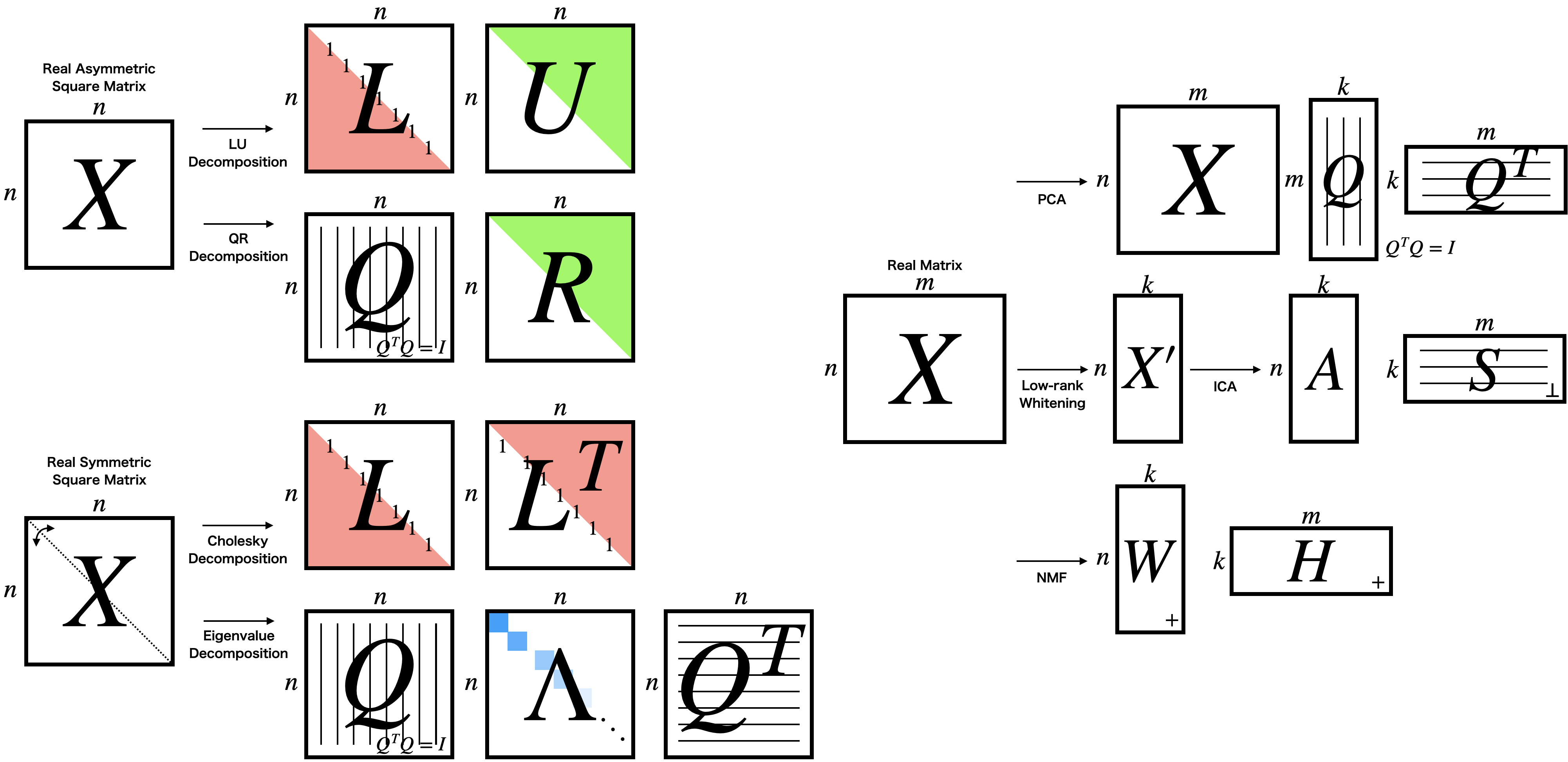
  • Real asymmetric square matrix（Tutorial 1）

    • LU Decomposition（Reference）

    • QR Decomposition（Reference）

  • Real symmetric square matrix（Tutorial 1）

    • Cholesky Decomposition（Reference）

    • Eigenvalue Decomposition（Reference）

  • Real matrix（Tutorial 2）

    • Principal Component Analysis (PCA, Reference）

      • Rec-mode (The high dimensional data is once projected to the lower dimensional space, and then is reconstructed to the original dimension)

      • Factor-mode (The variance of the score is maximized in the lower dimensional space)

    • Independent Component Analysis（ICA, Reference）

      • Kurtosis-based

      • Negentropy-based

      • Deep Deterministic ICA (DDICA, Reference）

    • Non-negative matrix（Tutorial 2）

      • Non-negative Matrix Factorization（NMF, Reference）

• Supervised Matrix Decomposition（Tutorial 3）

  • Partial Least Squares（PLS, Reference）

    • Rec-mode

    • Factor-mode

Reference

• LU/QR/Cholesky/Eigenvalue Decomposition

  • Gene H. Golub, Charles F. Van Loan Matrix Computations (Johns Hopkins Studies in the Mathematical Sciences)

• Principal Component Analysis (PCA) / Partial Least Squares (PLS)

  • R. Arora, A. Cotter, K. Livescu and N. Srebro, Stochastic optimization for PCA and PLS, 2012 50th Annual Allerton Conference on Communication, Control, and Computing, 2012, 861-868. 2012

• Independent Component Analysis (ICA)

  • Hybarinen, A. and Oja, E. Independent component analysis: algorithms and applications, Neural Networks, 13, 411-430. 2000

• Deep Deterministic ICA (DDICA)

  • H. Li, S. Yu and J. C. Príncipe, Deep Deterministic Independent Component Analysis for Hyperspectral Unmixing, 2022 IEEE International Conference on Acoustics, Speech and Signal Processing (ICASSP), 3878-3882, 2022

• Non-negative Matrix Factorization (NMF)

  • Kimura, K. A Study on Efficient Algorithms for Nonnegative Matrix/Tensor Factorization, Ph.D. Thesis, 2017

  • Exponent term depending on Beta parameter

    • Nakano, M. et al., Convergence-guaranteed multiplicative algorithms for nonnegative matrix factorization with Beta-divergence. IEEE MLSP, 283-288, 2010

  • Beta-divergence NMF and Backpropagation

    • https://yoyololicon.github.io/posts/2021/02/torchnmf-algorithm/